The Kaplan-Meier estimator is the standard nonparametric estimator of the survival function when data may be right-censored. It is also called the product-limit estimator because it is constructed by multiplying estimated conditional survival probabilities across event times.
2.1 Warm-Up: The Empirical Distribution Function Without Censoring
Before introducing censoring, it is helpful to recall the standard estimator of a distribution function when all event times are fully observed.
Suppose we observe independent event times \[
T_1, T_2, \dots, T_n
\] with no censoring. The distribution function is \[
F(t) = P(T \le t).
\] The natural estimator of \(F(t)\) is the empirical distribution function (EDF): \[
\widehat{F}(t)
=
\frac{1}{n}\sum_{i=1}^n I(T_i \le t).
\]
This estimator is simply the sample proportion of subjects whose event time is at or before time \(t\). The corresponding estimator of the survival function is \[
\widehat{S}(t) = 1 - \widehat{F}(t).
\]
Thus, when there is no censoring, estimating the survival curve is straightforward: at each time point \(t\), we just count the proportion of subjects who have survived beyond \(t\).
For example, suppose the observed event times are \[
2,\ 4,\ 5,\ 7,\ 8.
\] Then \[
\widehat{F}(5)=\frac{3}{5}=0.6,
\qquad
\widehat{S}(5)=1-\widehat{F}(5)=0.4.
\] This means that \(60\%\) of the sample has experienced the event by time 5, and \(40\%\) is still event-free beyond time 5.
The difficulty with censoring is that we can no longer directly count the proportion of subjects with \(T_i \le t\) or \(T_i > t\), because some lifetimes are only partially observed. The Kaplan-Meier estimator solves this problem by generalizing the same basic counting idea to the censored-data setting.
2.2 What Is the Kaplan-Meier Estimator?
Let \(T\) denote the event time and let \[
S(t) = P(T > t)
\] be the survival function. In practice, we usually observe \[
Y_i = \min(T_i, C_i), \qquad \Delta_i = I(T_i \le C_i),
\] where \(C_i\) is a censoring time, \(Y_i\) is the observed follow-up time, and \(\Delta_i\) indicates whether the event was observed.
Suppose the distinct observed event times are \[
t_{(1)} < t_{(2)} < \cdots < t_{(k)}.
\] Then we have the following decomposition of the survival function: \[
\begin{aligned}
&{S}(t_{(k)})\\
= &P(T>t_{(k)})\\
= &P(T>t_{(k)}|T>t_{(k-1)})P(T>t_{(k-1)})\\
= &P(T>t_{(k)}|T>t_{(k-1)})P(T>t_{(k-1)}|T>t_{(k-2)})\cdots P(T>t_{(2)}|T>t_{(1)})P(T>t_{(1)})\\
= & \prod_{j:t_{(j)}\leq t_{(k)}}P(T>t_{(j)}|T>t_{(j-1)}) \\
= & \prod_{j:t_{(j)}\leq t_{(k)}}(1-P(T=t_{(j)}|T\geq t_{(j)}) )\\
= & \prod_{j:t_{(j)}\leq t_{(k)}}(1-P(T=t_{(j)}|T\geq t_{(j)},C\geq t_{(j)} ) )\\
\end{aligned}
\]
At each event time \(t_{(j)}\), define
\(n_j\): the number of individuals still at risk just before time \(t_{(j)}\),
\(d_j\): the number of events occurring at time \(t_{(j)}\).
The Kaplan-Meier estimator of the survival function is (this is simply the plug-in principal) \[
\widehat{S}(t)
=
\prod_{j: t_{(j)} \le t}
\left(1 - \frac{d_j}{n_j}\right)
=
\prod_{j: t_{(j)} \le t}
\frac{n_j - d_j}{n_j}.
\]
This formula has a simple interpretation. At each event time, we estimate the conditional probability of surviving past that time by \[
\widehat{P}(T > t_{(j)} \mid T \ge t_{(j)}) = \frac{n_j - d_j}{n_j},
\] and then multiply these conditional survival probabilities together. Therefore, \[
\widehat{S}(t)
=
\prod_{j: t_{(j)} \le t}
\widehat{P}(T > t_{(j)} \mid T \ge t_{(j)}).
\]
Several important features follow directly from the definition:
\(\widehat{S}(t)\) is a step function.
It only drops at observed event times.
Censored observations do not cause vertical drops.
Censored observations do reduce the size of later risk sets.
No parametric form for the survival distribution is assumed.
2.2.1 The Key Assumption: Independent Censoring
The most important assumption behind the Kaplan-Meier estimator is independent censoring (also called non-informative censoring). Informally, this means that subjects who are censored at a given time should have the same future survival prospects as subjects who remain under observation at that time.
In a simple formulation, the event time \(T\) and censoring time \(C\) are assumed to be independent. More realistically, in many applications we assume they are independent conditional on the variables used in the analysis.
This assumption matters because the Kaplan-Meier estimator treats censored individuals as representative of those still at risk up to the moment of censoring. If censoring is related to prognosis, the estimator can be biased. For example, if very sick patients are more likely to drop out of follow-up, the Kaplan-Meier curve may overestimate survival.
In addition to independent censoring, it is usually assumed that:
subjects are independent of one another,
event and censoring times are measured accurately,
the survival experience of subjects recruited early and late in the study is comparable.
2.3 A Clinical Example
To see how the Kaplan-Meier estimator works, consider the follow-up times of seven patients in a small clinical study. The outcome is time from treatment to relapse, measured in months.
Table 2.1: A small survival dataset with right censoring.
Patient
Time (months)
Status
A
2
Relapse
B
3
Censored
C
4
Relapse
D
5
Relapse
E
5
Relapse
F
7
Relapse
G
9
Censored
The distinct event times are \(2\), \(4\), \(5\), and \(7\). Notice that two relapses occur at month 5. The censoring times occur at \(3\) and \(9\), but censoring times do not create jumps in the Kaplan-Meier curve.
We will use this example in the next section to show how the redistribute-to-the-right algorithm produces the Kaplan-Meier estimator by hand.
2.4 The Redistribute-to-the-Right Algorithm
An intuitive way to understand the Kaplan-Meier estimator is through the redistribute-to-the-right algorithm.
Start by assigning each subject equal probability mass \(1/n\). If an event is observed, that subject keeps its mass at the event time. If a subject is censored, then that subject’s probability mass cannot stay at the censoring time, because the event did not occur there. Instead, the censored subject’s mass is redistributed equally over the subjects who remain under observation at later times, that is, to the subjects to the right.
This idea explains why censoring does not cause a drop in the Kaplan-Meier curve. A censored subject is not counted as a failure. Rather, its weight is passed forward to those who are still at risk.
The algorithm can be described informally as follows:
Begin with probability mass \(1/n\) on each subject.
Move through the observed times from left to right.
When an event occurs, record the mass attached to that event time.
When a censoring time occurs, redistribute that subject’s mass equally among those still at risk later.
The estimated distribution function at time \(t\) is the total mass assigned to event times up to \(t\).
The estimated survival function is one minus this estimated distribution function.
This algorithm leads to exactly the Kaplan-Meier estimator. It is especially useful pedagogically because it connects the Kaplan-Meier curve to the empirical distribution function from the no-censoring setting.
To see the connection, notice the following:
If there is no censoring, no redistribution is needed.
Then each subject simply contributes mass \(1/n\) at its event time.
The resulting estimator is exactly the empirical distribution function.
With censoring, redistribution preserves the total probability mass while accounting for incomplete follow-up.
2.4.1 Applying the Algorithm to the Example in Section 4.3
Now apply the algorithm to the dataset in Table Table 2.1. Initially, each of the 7 patients receives probability mass \(1/7\).
Table 2.2: Redistribute-to-the-right calculation for the data in Table Table 2.1.
Time
Observation
Redistribution step
Event mass recorded
2
A relapses
A keeps its mass \(1/7\) at time 2
\(1/7\)
3
B is censored
B’s mass \(1/7\) is split equally among C, D, E, F, and G, so each receives an extra \(1/35\)
0
4
C relapses
C now carries mass \(1/7 + 1/35 = 6/35\) and keeps it at time 4
\(6/35\)
5
D and E relapse
D and E each carry mass \(6/35\), so the total event mass recorded at time 5 is \(12/35\)
\(12/35\)
7
F relapses
F carries mass \(6/35\) and keeps it at time 7
\(6/35\)
9
G is censored
G’s remaining mass \(6/35\) stays to the right of all observed event times
0
Therefore the estimated distribution function places masses \[
\frac{1}{7},\ \frac{6}{35},\ \frac{12}{35},\ \frac{6}{35}
\] at event times \(2\), \(4\), \(5\), and \(7\), respectively. Hence \[
\widehat{F}(2)=\frac{1}{7}, \qquad
\widehat{F}(4)=\frac{1}{7}+\frac{6}{35}=\frac{11}{35},
\]\[
\widehat{F}(5)=\frac{23}{35}, \qquad
\widehat{F}(7)=\frac{29}{35}.
\] Since \(\widehat{S}(t)=1-\widehat{F}(t)\), the Kaplan-Meier estimates are \[
\widehat{S}(2)=\frac{6}{7}, \qquad
\widehat{S}(4)=\frac{24}{35}, \qquad
\widehat{S}(5)=\frac{12}{35}, \qquad
\widehat{S}(7)=\frac{6}{35}.
\]
These values agree exactly with the product-limit formula:
Table 2.3: Kaplan-Meier calculation from the product-limit formula for the data in Table Table 2.1.
The resulting Kaplan-Meier curve is \[
\widehat{S}(t)
=
\begin{cases}
1, & 0 \le t < 2,\\[6pt]
\dfrac{6}{7}, & 2 \le t < 4,\\[8pt]
\dfrac{24}{35}, & 4 \le t < 5,\\[8pt]
\dfrac{12}{35}, & 5 \le t < 7,\\[8pt]
\dfrac{6}{35}, & t \ge 7.
\end{cases}
\]
Notice that the curve is flat between event times and drops only when a relapse is observed. The median survival time is the first time at which the estimated survival probability falls to \(0.5\) or below. Here, \[
\widehat{S}(4)=0.686 > 0.5
\qquad \text{and} \qquad
\widehat{S}(5)=0.343 < 0.5,
\] so the estimated median survival is 5 months.
2.5 Kaplan-Meier Estimation in R
The survival package in R provides the standard tools for Kaplan-Meier estimation. The next example uses the built-in lung dataset from that package. This dataset contains survival times for patients with advanced lung cancer.
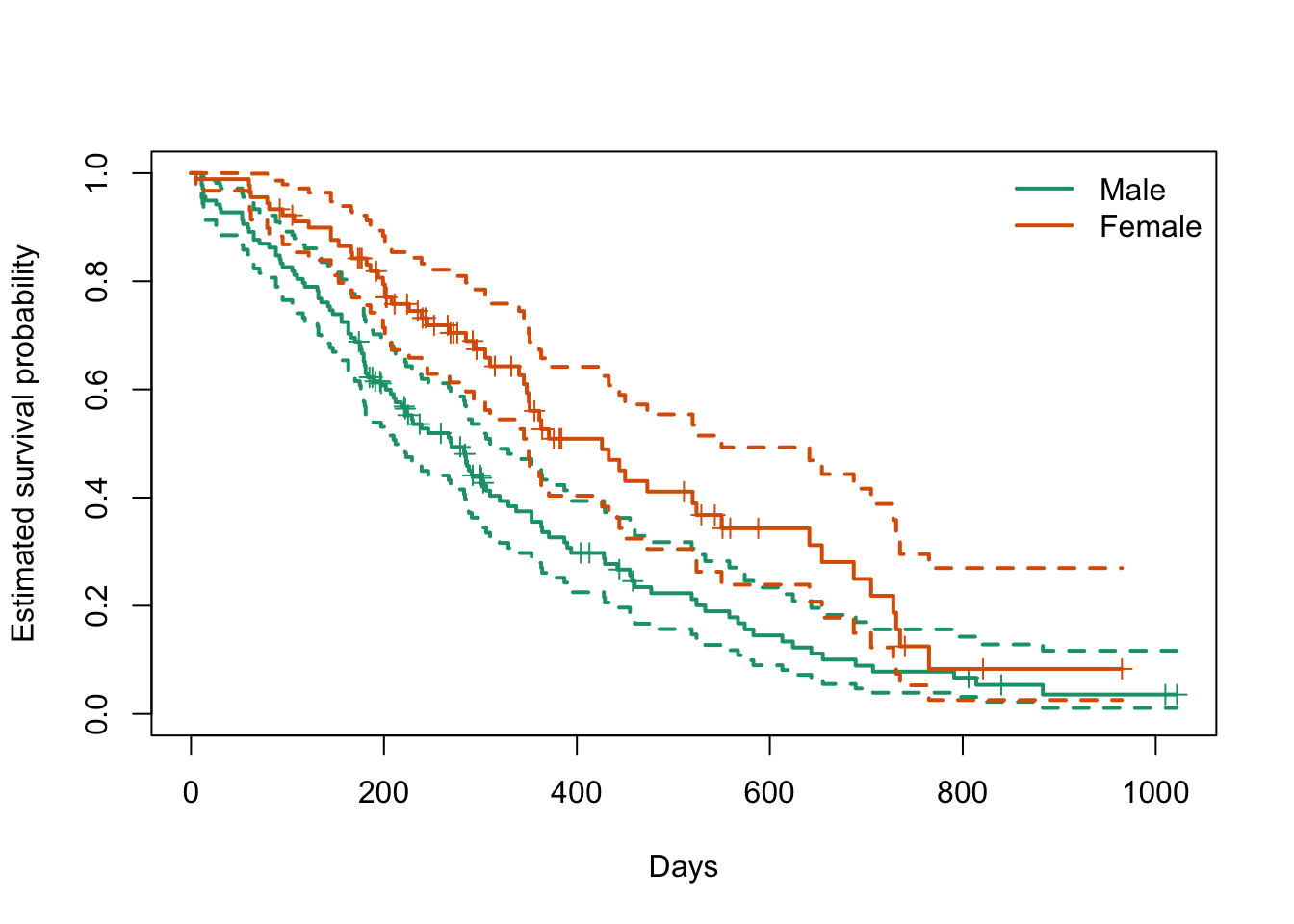
We will compare the Kaplan-Meier curves for males and females.
Kaplan-Meier curves for the lung dataset, grouped by sex.
Some key points to notice when reading the Kaplan-Meier plot are:
Each downward step corresponds to one or more observed deaths.
The short marks on the curves indicate censoring times.
The curve that stays higher indicates better estimated survival.
The curve becomes less stable in the right tail because fewer subjects remain at risk.
For this dataset, the female curve lies above the male curve for most of the follow-up period. This suggests that females have better observed survival than males in these data. The estimated median survival times are approximately 270 days for males and 426 days for females.
This interpretation should be kept descriptive. A Kaplan-Meier curve summarizes survival experience in the observed groups, but by itself it does not establish a causal effect. Group differences may also reflect other prognostic variables besides sex.
2.6 Variance of the Kaplan-Meier Estimator
Because the Kaplan-Meier curve is an estimate, it is important to quantify its uncertainty. The standard large-sample variance estimator is Greenwood’s formula: \[
\widehat{\mathrm{Var}}\{\widehat{S}(t)\}
=
\widehat{S}(t)^2
\sum_{j: t_{(j)} \le t}
\frac{d_j}{n_j(n_j-d_j)}.
\]
The corresponding estimated standard error is \[
\widehat{\mathrm{se}}\{\widehat{S}(t)\}
=
\sqrt{
\widehat{\mathrm{Var}}\{\widehat{S}(t)\}
}.
\]
2.6.1 Intuition for Greenwood’s Formula
Greenwood’s formula is easier to understand if we focus on what happens at each event time.
The Kaplan-Meier estimator is a product of many conditional survival factors.
Each factor \(\left(1-d_j/n_j\right)\) is estimated with some uncertainty.
The term \(\dfrac{d_j}{n_j(n_j-d_j)}\) measures how much uncertainty is contributed by the \(j\)th event time.
Large risk sets make this term small, so early parts of the curve are usually estimated more precisely.
Small risk sets make this term large, so the tail of the curve is often much more variable.
The multiplier \(\widehat{S}(t)^2\) appears because the variance is being translated back to the survival scale after combining the uncertainty from the product of conditional survival probabilities.
For the hand-worked example above, at time \(t=7\) we found \[
\widehat{S}(7)=\frac{6}{35}.
\] Greenwood’s formula gives \[
\widehat{\mathrm{Var}}\{\widehat{S}(7)\}
=
\left(\frac{6}{35}\right)^2
\left(
\frac{1}{7\cdot 6}
+
\frac{1}{5\cdot 4}
+
\frac{2}{4\cdot 2}
+
\frac{1}{2\cdot 1}
\right)
\approx 0.024.
\] Thus the estimated standard error is approximately \[
\widehat{\mathrm{se}}\{\widehat{S}(7)\}
\approx \sqrt{0.024}
\approx 0.156.
\]
The uncertainty is still substantial near the end of follow-up because only 2 patients were still at risk just before month 7. The tied failures at month 5 also make a noticeable contribution through the term \(\frac{2}{4\cdot 2}\). This is exactly the pattern seen in practice: the right tail of a Kaplan-Meier curve is usually the noisiest part, especially when the risk set is small or multiple events occur at the same time.
In applications, Greenwood’s formula is commonly used to construct confidence intervals for the survival function. Many software packages, including survival in R, use a transformed scale such as the log-log scale to obtain intervals that remain within \([0,1]\).
2.7 The Nelson-Aalen Estimator
The Kaplan-Meier estimator focuses on the survival function. Another important nonparametric estimator in survival analysis is the Nelson-Aalen estimator, which estimates the cumulative hazard function \[
\Lambda(t) = \int_0^t \lambda(u)\,du.
\]
If the distinct event times are \(t_{(1)} < \cdots < t_{(k)}\), with \(n_j\) subjects at risk and \(d_j\) events at time \(t_{(j)}\), then the Nelson-Aalen estimator is \[
\widehat{\Lambda}_{NA}(t)
=
\sum_{j:t_{(j)}\le t} \frac{d_j}{n_j}.
\]
This estimator is very natural: at each event time we add the observed hazard increment \(d_j/n_j\), and then accumulate these increments over time. Thus, unlike the Kaplan-Meier estimator, which is multiplicative, the Nelson-Aalen estimator is additive.
Several basic properties are worth noting:
\(\widehat{\Lambda}_{NA}(t)\) is a step function.
It only jumps at observed event times.
The jump size at time \(t_{(j)}\) is \(d_j/n_j\).
Censoring changes later risk sets but does not itself create a jump.
For the hand-worked example above, the event times are \(2\), \(4\), \(5\), and \(7\), with \[
(n_j,d_j) = (7,1),\ (5,1),\ (4,2),\ (2,1).
\] Therefore \[
\widehat{\Lambda}_{NA}(7)
=
\frac{1}{7}+\frac{1}{5}+\frac{2}{4}+\frac{1}{2}
=
\frac{47}{35}
\approx 1.343.
\]
If we want a survival estimate based on the cumulative hazard, we can combine the Nelson-Aalen estimator with the identity \[
S(t)=\exp\{-\Lambda(t)\}
\] to obtain \[
\widehat{S}_{NA}(t)=\exp\big\{-\widehat{\Lambda}_{NA}(t)\big\}.
\] For the same example, \[
\widehat{S}_{NA}(7)
=
\exp\left(-\frac{47}{35}\right)
\approx 0.261.
\]
This differs from the Kaplan-Meier estimate \(\widehat{S}(7)=6/35\approx 0.171\), because the sample is small and the hazard jumps are fairly large. In larger samples, or when the increments \(d_j/n_j\) are small, the two approaches are often quite close. Indeed, \[
\log \widehat{S}_{KM}(t)
=
\sum_{j:t_{(j)}\le t}\log\left(1-\frac{d_j}{n_j}\right)
\approx
-\sum_{j:t_{(j)}\le t}\frac{d_j}{n_j}
=
-\widehat{\Lambda}_{NA}(t),
\] so the Kaplan-Meier and Nelson-Aalen estimators are closely related.
The Nelson-Aalen estimator is especially useful because cumulative hazards are often easier to manipulate mathematically than survival functions. It also appears naturally in later topics such as the log-rank test and the Cox proportional hazards model.
2.8 Summary
The Kaplan-Meier estimator is the basic nonparametric tool for estimating a survival curve from right-censored data. It is obtained by multiplying conditional survival probabilities across event times. Its validity depends crucially on the assumption of independent censoring. In practice, the estimator is easy to compute by hand for a small dataset and easy to fit in R using survfit(). Greenwood’s formula provides the standard variance estimator and helps explain why uncertainty increases when only a few subjects remain at risk. The Nelson-Aalen estimator gives a closely related nonparametric estimator of the cumulative hazard function and provides another important way to summarize censored survival data.